Why fleet size affects haulage: utilisation and profit

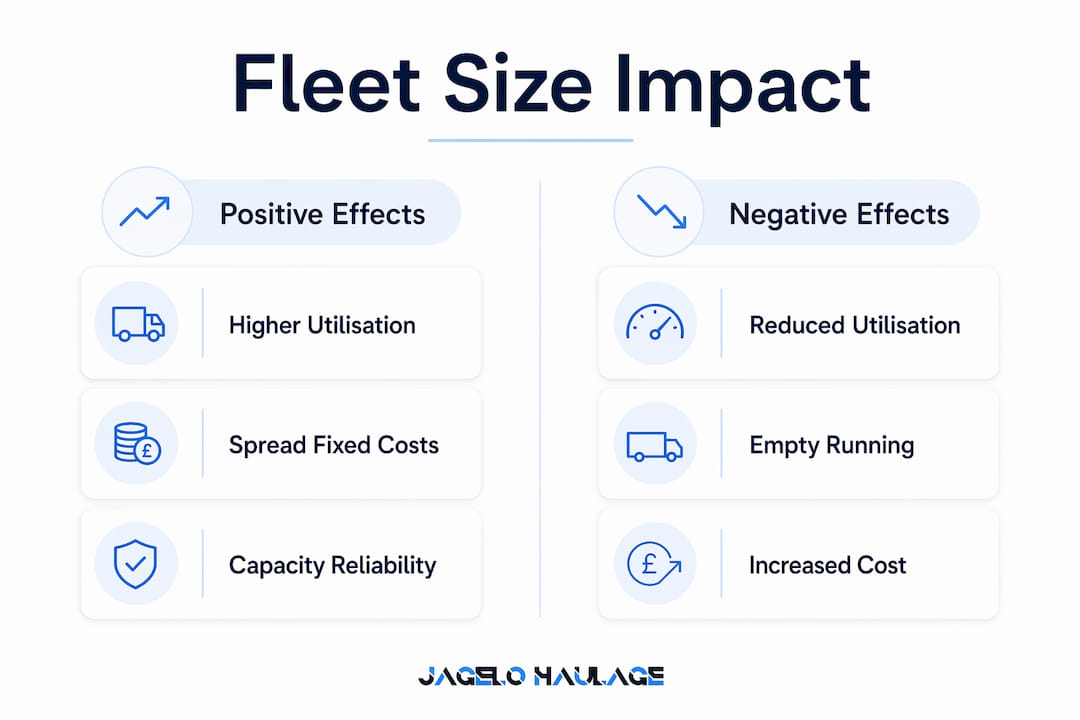
Fleet size alters haulage profitability and service reliability by changing three interlocked variables: vehicle utilisation rate, empty kilometres run, and fixed cost exposure per active unit. Get the balance wrong in either direction and the consequences compound quickly. An oversized fleet inflates standing costs through depreciation, insurance and maintenance on idle assets; an undersized fleet forces expensive emergency subcontracting, damages service levels and erodes client confidence. The impact of fleet size on a UK container-haulage operation is therefore not a procurement question but a continuous operational discipline.
The core mechanisms at a glance:
- Utilisation rate: adding vehicles without matching demand dilutes the percentage of time each unit is productively loaded and moving, raising cost per kilometre.
- Empty running: a fleet larger than demand requires generates more dead-leg kilometres as vehicles reposition without revenue-generating cargo.
- Spare ratio: the proportion of vehicles held in reserve for maintenance and contingency must be tuned to duty cycle and fleet age, not set as a fixed industry constant.
- Fixed vs variable costs: depreciation, insurance and standing maintenance are fixed per vehicle regardless of activity; the fewer kilometres each vehicle covers, the higher those costs sit per kilometre.
- Quick rule of thumb: if your fleet utilisation rate drops below typical industry thresholds of available vehicle-days on a sustained basis, your fixed cost per job is likely rising faster than any service-level benefit justifies.
The most actionable sections for immediate use are the KPI formulas and worked calculation in the measuring and modelling section, the spare-capacity tactics table, and the decision checklist for buy-versus-contract choices.
Table of Contents
- What does ‘fleet size’ actually mean in haulage?
- How fleet size changes your operational levers
- Why adding trucks eventually stops improving productivity
- How to measure and model fleet-size decisions
- How to manage spare capacity without owning idle assets
- Does technology actually reduce the number of vehicles you need?
- A UK container-haulage operator’s sizing intervention
- Buy, lease, or contract? A decision checklist for fleet capacity
- What UK fleet managers should do next
- Key takeaways
- The trade-off most fleet managers accept too quietly
- Contracted capacity as an alternative to owning peak vehicles
- Useful sources for fleet-sizing analysis
What does ‘fleet size’ actually mean in haulage?
Fleet size is not simply a count of trucks. For modelling and management purposes, it encompasses every resource category that determines how many jobs a fleet can complete in a given period.
Active units are vehicles available for dispatch on any given day, excluding those in scheduled maintenance, awaiting repair, or undergoing compliance inspection. Idle or spare units are those held in reserve to cover breakdowns, planned maintenance windows, and demand spikes. The trailer pool is counted separately from tractor units in container haulage, because a single tractor can cycle through multiple trailers in a day, and trailer availability often constrains throughput before tractor availability does. Driver headcount must account for shift patterns, Working Time Directive compliance, and multi-shift operations, since a vehicle is operationally unavailable without a compliant driver regardless of its mechanical status.
Scope boundaries matter too. Owned capacity and contracted capacity (subcontractors, spot-hire) serve different cost and control profiles and should be tracked separately in any sizing model. Specialised units, including ADR-certified vehicles for hazardous goods, temperature-controlled trailers for refrigerated cargo, and abnormal-load configurations for oversized freight, follow different utilisation and spare-ratio rules because their duty cycles, compliance requirements, and replacement lead times differ from standard curtainsiders or skeletal trailers.
| Term | Definition | Measurement unit used in modelling |
|---|---|---|
| Active units | Vehicles available for dispatch on a given day | Count (daily average) |
| Spare ratio | Idle/reserve vehicles as a proportion of total fleet | Percentage (%) |
| Utilisation rate | Productive vehicle-days as a proportion of available vehicle-days | Percentage (%) |
| Empty km | Kilometres driven without revenue-generating cargo | km per completed job |
| Turnaround time | Total cycle time from port gate-in to gate-out and return | Hours per cycle |
| Trailer pool ratio | Trailers per tractor unit | Ratio (e.g. 1.4:1) |
| Driver availability | Compliant drivers available relative to active units | Percentage (%) |
In container haulage specifically, the most precise measure of capacity is not raw vehicle count but cycle time: the total elapsed time from port gate-in, through loaded transit, to empty return or next collection. Reducing cycle time increases the number of jobs each vehicle can complete per week, which means a smaller fleet can serve the same volume. ISO fleet management guidance confirms that centralising tracking and maintenance analytics around cycle-time data drives measurable efficiency gains that a simple headcount metric would miss entirely.
How fleet size changes your operational levers
The causal pathways from fleet size to profitability run through several interlocked mechanisms. Understanding each one tells you which lever to pull first.
Utilisation rate falls as fleet size grows beyond demand. Every vehicle added to a fleet that cannot absorb the additional capacity reduces the average utilisation rate across the whole fleet. A fleet of 20 vehicles completing 16 vehicle-days of productive work per day runs at 80% utilisation. Add four more vehicles without adding demand and utilisation drops to 64%. Fixed costs per vehicle remain constant, so cost per productive kilometre rises.

Empty running increases with spare capacity. Vehicles that cannot be loaded on a return leg run empty kilometres that consume fuel, driver hours and tyre wear without generating revenue. Fleet optimisation converts real-time data into prescriptive routing decisions that reduce empty running, but the structural cause is a mismatch between fleet size and demand density on specific corridors. In port-to-door container haulage, one-way contract structures and port-centric routing make backhaul opportunities structurally limited, which means empty-km management is a more acute problem than in general haulage.
Fixed costs per vehicle spread differently at different utilisation levels. Depreciation, insurance, vehicle excise duty and standing maintenance are fixed regardless of how many kilometres a vehicle covers. As utilisation falls, those fixed costs are divided across fewer productive kilometres, raising cost per km. Fuel costs represent 20–30% of total fleet operating expenses, making them the largest variable component, but it is the fixed-cost leverage that makes utilisation the primary profitability driver.

Dwell time at terminals constrains effective capacity more than raw vehicle count. In port operations, a vehicle waiting two hours at a terminal gate is operationally unavailable for that period. Reducing dwell time through pre-booking, Vehicle Booking System (VBS) compliance and optimised slot management increases the number of cycles each vehicle completes per week, effectively expanding capacity without adding trucks. The relationship between haulage scheduling and warehouse throughput follows the same logic: a tighter booking discipline raises cycle frequency and reduces required fleet size.
Service reliability has a non-linear relationship with spare ratio. A fleet with zero spare vehicles is highly exposed to any mechanical failure or driver absence. Adding one or two spare units dramatically improves service reliability. Adding a fifth or sixth spare unit beyond what maintenance schedules require produces negligible further reliability improvement while adding fixed cost.
- Fleet size above demand: utilisation falls, cost per km rises, empty km increases.
- Fleet size below demand: service failures increase, emergency subcontracting costs spike, demurrage and detention charges accumulate.
- Optimal range: utilisation maximised, spare ratio tuned to duty cycle, empty km minimised through routing discipline.
- Dwell time reduction at port: often delivers more effective capacity than adding a vehicle.
Pro Tip: Before purchasing an additional vehicle to resolve a service failure, audit dwell time and turnaround data first. In container haulage, a one-hour reduction in average port dwell time per cycle can recover the equivalent of one additional vehicle-day per week across a fleet of ten units.
Why adding trucks eventually stops improving productivity
The relationship between fleet size and operational performance is non-linear. Up to a point, each additional vehicle adds roughly proportional capacity. Beyond that point, marginal gains fall sharply while marginal costs continue to accumulate.
The operational causes of diminishing returns are well understood. As fleet size grows, routing becomes more complex: more vehicles competing for the same collection windows, terminal slots and delivery appointments create scheduling conflicts that erode the efficiency gains each new unit was supposed to deliver. Empty kilometres grow because demand density on specific corridors does not scale with fleet size. Management overhead increases as supervisory span widens, compliance monitoring becomes more demanding, and driver performance variability rises.
Academic simulation and queueing research consistently demonstrates this non-linear pattern: fleet availability produces roughly linear benefit up to a threshold, after which marginal gains fall sharply and waiting-time improvements plateau. AIMMS recommends modelling fleet size across demand ranges rather than sizing for averages or peaks alone, precisely because the cost curve is not symmetric.
Sizing a fleet for average demand leaves you short at peak periods. Sizing for peak demand creates chronic underutilisation for the majority of the year. The minimum total-cost solution almost always lies between those two points, and finding it requires modelling the demand distribution, not just its mean or maximum.
A simple worked example illustrates the fixed-cost leverage:
- Baseline: 10 vehicles, each covering 4,000 km per month. Fixed cost per vehicle: £2,000/month. Variable cost: £0.30/km. Total monthly cost: £(10 × 2,000) + £(10 × 4,000 × 0.30) = £20,000 + £12,000 = £32,000. Cost per km: £0.80.
- Add 2 vehicles, demand unchanged: 12 vehicles, each now covering 3,333 km/month (same total demand spread across more units). Total monthly cost: £(12 × 2,000) + £(12 × 3,333 × 0.30) = £24,000 + £12,000 = £36,000. Cost per km: £0.90.
- Net effect: adding 20% more vehicles with no demand increase raises cost per km by 12.5% and total monthly cost by £4,000, with no service improvement.
The point of diminishing returns is not a single number but a range that depends on demand variability, route structure and spare-ratio requirements. Sensitivity analysis across two or three demand scenarios, run in a spreadsheet or a dedicated fleet size optimisation model, will locate that range more reliably than any rule of thumb.
How to measure and model fleet-size decisions
Effective sizing decisions rest on a small set of KPIs that are both measurable from existing data sources and directly linked to profitability. The formulas below are replicable from telematics, transport management system (TMS) data and management accounts.
Core KPIs and their formulas
| KPI | Formula | Required inputs | Data source |
|---|---|---|---|
| Utilisation rate | (Productive vehicle-days ÷ Available vehicle-days) × 100 | Dispatch records, maintenance logs | TMS / telematics |
| Empty km per job | Total empty km ÷ Number of completed jobs | GPS mileage, job completion records | Telematics / TMS |
| Cost per km | Total fleet cost ÷ Total km driven | Fuel, maintenance, depreciation, insurance | Accounts / telematics |
| Cost per job | Total fleet cost ÷ Number of completed jobs | All cost lines, job count | Accounts / TMS |
| Average turnaround | Sum of cycle times ÷ Number of cycles | Gate-in/gate-out timestamps, delivery POD | Port VBS / TMS |
| Spare ratio | (Spare vehicles ÷ Total fleet) × 100 | Fleet register, maintenance schedule | Fleet register |
Real-time tracking and analytics centralise these inputs and make weekly KPI reporting practical even for mid-sized fleets. Geotab’s utilisation reporting approach, for instance, uses telematics data to identify idle assets that can be reassigned or removed from the active fleet, directly reducing fixed cost exposure.
Pro Tip: Pair the utilisation rate with the spare ratio in a single weekly dashboard. A utilisation rate above 85% with a spare ratio below 8% is a warning sign: you are running too lean and one breakdown or driver absence away from a service failure. A utilisation rate below 75–80% with a spare ratio above 20% signals chronic oversizing.
Step-by-step sizing simulation
- Collect baseline data: gather 12 weeks of job volume, vehicle-days dispatched, empty km, and cycle times from your TMS and telematics.
- Calculate baseline KPIs: compute utilisation rate, cost per km, cost per job and average turnaround using the formulas above.
- Define demand scenarios: model three demand levels: current average, peak (highest four-week period), and a 15% growth scenario.
- Set spare-ratio assumptions: determine the maintenance-driven minimum spare ratio for your fleet age profile. Older fleets require a higher spare ratio than newer ones.
- Run scenario outputs: for each demand scenario, calculate the fleet size required to maintain your target utilisation rate (e.g. 78–82%) at the defined spare ratio.
- Evaluate the gap: compare required fleet size against current fleet size. The gap defines whether you are over- or under-provisioned and by how much.
Worked utilisation-to-cost conversion: if a fleet currently running at moderate utilisation can achieve the same output with fewer vehicles if utilisation improves, resulting in cost savings in fixed costs per vehicle without reducing throughput. That is the arithmetic case for capacity planning as a cost-reduction discipline.
How to manage spare capacity without owning idle assets
The practical challenge for most UK haulage operators is not identifying the optimal fleet size in theory but managing the gap between owned capacity and actual demand in real time. Several tactical options exist, each with a distinct cost profile, control level and compliance risk.
Pro Tip: Set a utilisation threshold trigger before you need it. When utilisation drops below 75–80% for three consecutive weeks, that is the signal to activate subcontractor capacity rather than waiting for a service failure to force the decision.
| Tactic | Cost profile | Control level | Reliability | Compliance risk |
|---|---|---|---|---|
| Long-term vehicle lease | Fixed monthly cost, lower than ownership | High (your drivers, your processes) | High | Low (operator licence covers leased vehicles) |
| Flexible driver contracts | Variable cost, scales with demand | Medium (agency drivers, variable familiarity) | Medium | Medium (agency compliance varies) |
| Approved subcontractor panel | Variable, per-job rate | Lower (third-party processes) | Medium-High (if panel is audited) | Medium (O-licence, insurance verification required) |
| Spot-hire capacity | Highest per-job cost | Lowest | Variable | Higher (ad hoc vetting) |
| Fleet pooling / multi-client sharing | Shared fixed cost, complex to administer | Medium | Medium | Medium (requires contractual framework) |
The core-and-flex model is the most widely adopted approach among UK operators managing seasonal or contract-driven demand variability. The principle is straightforward: maintain a core owned fleet sized for predictable baseline demand, and meet peaks with an audited subcontractor panel rather than owning for peak. This keeps fixed cost exposure proportional to the minimum reliable demand level while preserving service capacity for peaks. Merchant haulage arrangements add a further dimension: when the shipper controls the haulage contract, the operator must absorb demand variability that the shipping line would otherwise manage, making the subcontractor panel more critical.
Backhaul optimisation is a related tactic. In container haulage, where one-way port collections dominate, securing return loads or triangulated routes reduces empty km without adding vehicles. The commercial constraint is that port-centric operations often lack the network density to fill return legs consistently, which is why subcontractor panels and load-exchange arrangements tend to be more practical than internal backhaul programmes for operators focused on port logistics.
Implementation triggers worth setting in advance:
- Utilisation below 75–80% for three consecutive weeks: review for asset disposal or subcontractor activation.
- Utilisation above 88% for two consecutive weeks: assess whether contracted capacity or a leased unit is more cost-effective than a permanent addition.
- Spare ratio below 8%: review maintenance scheduling and consider a short-term lease to cover planned downtime.
Does technology actually reduce the number of vehicles you need?
The short answer is yes, but only when technology is paired with disciplined operational processes. ISO’s fleet management framework is explicit on this point: firms that combine telematics with structured processes gain the greatest utilisation improvements, while those that deploy technology without changing workflows see limited benefit.
The distinction between fleet management and fleet optimisation is worth stating precisely. Fleet management keeps assets running: it covers maintenance scheduling, compliance tracking, driver hours monitoring and basic GPS visibility. Fleet optimisation goes further, using continuous solver-driven re-planning to actively reassign vehicles and tasks in real time, reducing required fleet size by eliminating the slack that reactive management builds in as a buffer. Autofleet’s analysis of this distinction shows that many tools report utilisation retrospectively but do not change the immediate allocation of vehicles and tasks. True optimisation requires a decision engine, not just a dashboard.
The technology capabilities that materially reduce required vehicle counts, in order of implementation priority:
- Real-time GPS tracking: provides the visibility foundation for all other capabilities; without accurate location data, routing and utilisation analysis are unreliable.
- Dynamic route optimisation: reduces empty km and improves cycle frequency by recalculating routes as conditions change, rather than locking in plans at the start of a shift.
- Predictive maintenance: reduces unplanned downtime by flagging component wear before failure, which lowers the spare ratio required to maintain service levels.
- Driver performance analytics: identifies fuel-wasting behaviours (harsh braking, excessive idling, speeding) that inflate variable costs and accelerate vehicle wear.
- TMS integration with port VBS: synchronises terminal slot bookings with vehicle dispatch, reducing dwell time and improving cycle-time predictability.
Parts standardisation across the fleet also reduces maintenance downtime. Standardised truck parts reduce the number of unique components held in stock, shorten repair turnaround times and lower the spare ratio needed to cover unplanned failures. This is a frequently overlooked lever in fleet-size discussions.
Pro Tip: Sequence your technology roll-out: GPS tracking first, then TMS integration, then dynamic routing. Each layer depends on data quality from the previous one. Deploying route optimisation before your tracking data is clean produces worse routing decisions than a competent dispatcher working from experience.
A UK container-haulage operator’s sizing intervention
The following scenario illustrates how the principles above play out in a port-focused UK operation. The situation, intervention and metrics reflect the operational patterns common to container haulage at major UK ports including Felixstowe, Tilbury and Southampton.
Situation: A mid-sized UK container-haulage operator running 18 skeletal tractor units found that utilisation had drifted to approximately 68% over a 16-week period. The primary causes were a combination of an oversized spare ratio (four vehicles held as reserve, representing 22% of the fleet) and average port dwell times of 2.5 hours per visit, driven by inconsistent VBS slot compliance. Cost per container move had risen as fixed costs spread across fewer productive cycles.
Intervention and timeline: Over a 12-week period, the operator implemented three changes. First, they tightened VBS slot compliance through pre-booking discipline and driver briefings, reducing average dwell time to 1.4 hours. Second, they introduced a weekly utilisation review using telematics data, identifying two vehicles that had not completed a revenue job in 14 days. Third, they moved those two vehicles to a flexible lease arrangement, reducing the owned fleet to 16 units while retaining access to the two leased units during peak periods.
Reducing average port dwell time by one hour per cycle, across 16 vehicles completing two cycles per day, recovers the equivalent of 16 vehicle-hours of productive capacity daily. That is more effective capacity than adding a single new vehicle, at a fraction of the cost.
Before/after metrics (indicative):
- Utilisation rate: approximately 68% before, approximately 81% after.
- Average port dwell time: 2.5 hours before, 1.4 hours after.
- Spare ratio: 22% before, 12.5% after (two vehicles moved to flexible lease).
- Cost per container move: reduced as fixed costs spread across more productive cycles.
Replication checklist for other operators:
- Pull 12 weeks of telematics data and calculate current utilisation rate and spare ratio.
- Audit port dwell time by terminal and by driver; identify the highest-dwell outliers.
- Review VBS slot compliance rate; set a target of 90%+ pre-booked slots.
- Identify vehicles with fewer than two revenue jobs per week over the past four weeks.
- Model the cost impact of moving those vehicles to a flexible lease or subcontractor arrangement.
- Set weekly KPI review cadence: utilisation, dwell time, empty km per job.
For deeper context on port-to-door operations and container haulage practices at UK terminals, the strategic reference guide covers the operational detail behind these decisions.
Buy, lease, or contract? A decision checklist for fleet capacity
The marginal cost comparison between owned, leased and contracted capacity is the arithmetic foundation of any sizing decision. The checklist below structures the questions you need to answer before adding or shedding vehicles.
- What is the demand profile? Is demand steady, seasonal, or contract-driven with defined peaks? Steady demand favours ownership; variable demand favours a core-and-flex model.
- What is the service criticality? Does a missed collection trigger demurrage or detention charges? High service criticality raises the cost of under-provision and justifies a higher spare ratio or a contracted backup panel.
- What are the working capital constraints? Vehicle acquisition ties up capital and creates long-term depreciation obligations. Leasing converts capital expenditure to operating expenditure and preserves liquidity.
- What are the regulatory and security requirements? ADR certification, temperature-controlled compliance, and port security clearances limit which subcontractors can be used. If your specialist unit requirements are high, owned capacity may be unavoidable for those categories.
- What is the marginal cost of the next vehicle? Use this formula: Marginal cost per job (owned) = (Annual fixed cost per vehicle ÷ Annual jobs per vehicle) + Variable cost per job. Compare against the contracted rate per job from your subcontractor panel. If the contracted rate is lower than the owned marginal cost at your current utilisation level, contracting is cheaper.
- What is the fleet age profile? Older vehicles carry higher maintenance costs, lower residual values and greater spare-ratio requirements. An ageing fleet may justify replacement rather than addition.
- What does your TMS data show about peak frequency? If peak demand occurs for fewer than eight weeks per year, owning for peak is almost certainly more expensive than contracting for those weeks.
A container haulage partner selection checklist provides the procurement-side framework for auditing subcontractors before adding them to an approved panel, which is the prerequisite for making the contracted-capacity option reliable enough to depend on.
For linehaul operations specifically, understanding linehaul driver models and duty cycles informs how fleet composition decisions interact with driver contract structures, particularly when modelling multi-shift or overnight operations.
What UK fleet managers should do next
Three prioritised actions cover the most common gaps in fleet-size discipline among UK haulage operators.
- Measure first. Calculate your current utilisation rate, spare ratio and cost per km from the last 12 weeks of data. Most operators discover their utilisation is lower than assumed and their spare ratio is higher than maintenance schedules justify. The measurement itself often reveals the action.
- Model before you buy or cut. Run the three-scenario simulation (average demand, peak, growth) before adding or removing a vehicle. The worked arithmetic in the measuring and modelling section above takes less than an hour with TMS and accounts data. A decision made without this model is a guess.
- Discipline the spare ratio. Set the spare ratio as a tuning parameter reviewed quarterly, not a fixed number inherited from a previous fleet manager. A fleet of newer vehicles with predictable maintenance cycles can run a lower spare ratio than an ageing mixed fleet. The right number depends on your duty cycle, fleet age and subcontractor panel reliability.
As a final rule of thumb: if your spare ratio exceeds 15% and your utilisation rate is below 75–80% simultaneously, the commercial case for activating contracted capacity and reducing owned fleet size is almost always positive. The role of haulage in supply chain efficiency extends beyond cost management to service reliability, so any sizing decision must weigh both dimensions before committing.
Key takeaways
Fleet size primarily affects haulage profitability through three mechanisms: utilisation rate, empty kilometres, and fixed cost exposure per vehicle, all of which compound when fleet size and demand are misaligned.
| Point | Details |
|---|---|
| Utilisation drives cost per km | A utilisation rate below 75–80% raises fixed cost per km faster than any service benefit justifies. |
| Diminishing returns are real | Adding vehicles beyond demand increases total cost without improving throughput, as the worked example shows. |
| Dwell time beats headcount | Reducing port dwell time by one hour per cycle recovers more effective capacity than adding a vehicle. |
| Core-and-flex reduces risk | Sizing the owned fleet for baseline demand and contracting for peaks minimises fixed cost exposure. |
| Jhaulage for contracted peaks | Jhaulage operates a GPS-tracked fleet of over 40 units across major UK ports, providing audited contracted capacity for operators managing demand variability. |
The trade-off most fleet managers accept too quietly
Fleet sizing conversations in UK haulage almost always get framed as a capital question: how many vehicles can we afford? That framing is wrong, and it consistently leads operators to carry more owned capacity than they need.
The more useful frame is a utilisation question: at what fleet size does our cost per container move reach its minimum, given our actual demand distribution? Those are different questions with different answers, and the gap between them is where most of the avoidable cost sits. Operators who size for capital affordability tend to over-provision, accept low utilisation as normal, and then compensate by running older vehicles longer to defer replacement costs, which raises maintenance spend and spare-ratio requirements simultaneously.
The operational red flag that should trigger a sizing review is not a service failure. It is three consecutive weeks of utilisation below 75–80% without a clear seasonal explanation. By the time a service failure occurs, the fleet is already undersized for a different reason, and the response is reactive rather than planned. The discipline is in catching the utilisation signal early, running the scenario model, and making a deliberate decision about whether to activate contracted capacity, adjust the spare ratio, or accept a temporary cost increase while demand recovers.
Contracted capacity as an alternative to owning peak vehicles
When demand variability makes owning for peak commercially indefensible, contracted haulage with a specialist port operator is the most direct alternative. Jhaulage provides GPS-tracked container transport across the UK’s major ports, including Felixstowe, Tilbury, Southampton and Liverpool, with 24/7 operational support and a fleet of over 40 modern tractor units. For operators managing seasonal peaks, new contract wins or short-term demand surges, Jhaulage offers the port expertise and tracking infrastructure of an owned fleet without the capital commitment.
The practical benefit is straightforward: you access audited, compliant capacity with real-time visibility, without adding to your fixed cost base or extending your operator licence obligations. For freight forwarders, importers and logistics operators whose container volumes fluctuate, this is the arithmetic case for contracted container haulage as a complement to a right-sized owned fleet. Contact Jhaulage to discuss a capacity assessment for your peak periods or new port corridors.
Useful sources for fleet-sizing analysis
The resources below provide the analytical foundations and operational frameworks referenced throughout this article.
- ISO fleet management guidance: covers tracking, maintenance management and analytics as the standards basis for fleet efficiency measurement; directly relevant to KPI design and technology sequencing.
- AIMMS fleet size and composition modelling: explains how to model owned versus contracted cost curves across demand ranges; the primary reference for the diminishing-returns and scenario-modelling sections.
- Autofleet: fleet management optimisation: distinguishes reactive fleet management from continuous optimisation and explains the decision-engine capability required for real utilisation improvement.
- Geotab fleet management tips: practical guidance on utilisation reporting and seasonal asset reviews; useful for operators building their first KPI dashboard.
- Academia.edu: Finding the optimum fleet size of hauling trucks: simulation-based research demonstrating that cycle time and loading constraints determine the optimum fleet size; supports the diminishing-returns analysis.
- Autosist: complete guide to fleet operations: operational efficiency framework covering fuel cost benchmarks, maintenance discipline and real-time visibility; useful for fleet managers building an efficiency baseline.
- Jhaulage: logistics fleet management best practices: covers GPS tracking, telematics and route optimisation in the context of UK container haulage; the practical companion to the technology section of this article.
- Jhaulage: haulage capacity planning guide: step-by-step capacity planning methodology for logistics managers; pairs directly with the measuring and modelling section.